
Over the past three decades, the economic trajectories of India, China, Germany, Canada, and the United States have diverged sharply. China delivered the fastest sustained real-growth performance of the five, followed by India. The United States grew more slowly but with considerably greater consistency than its other advanced-economy peers. Canada remained a middling performer, while Germany recorded the weakest long-term growth and has entered the 2020s in an especially difficult position.
Using annual real GDP growth data for approximately 1995 through 2024, the contrast is striking. China averaged roughly 8.4% annual real GDP growth, India approximately 6.3%, the United States about 2.5%, Canada roughly 2.4%, and Germany only about 1.2%. These are simple averages of annual growth rates rather than cumulative growth rates. The International Monetary Fund (IMF) also notes that India’s World Economic Outlook data are presented on a fiscal-year basis, whereas the other economies are generally reported on a calendar-year basis, which should be considered when making precise annual comparisons (International Monetary Fund [IMF], 2026).
| Country | Approx. average annual real GDP growth, 1995–2024 |
|---|---|
| China | 8.4% |
| India | 6.3% |
| United States | 2.5% |
| Canada | 2.4% |
| Germany | 1.2% |
These differences may appear modest when expressed as annual percentages, but they compound dramatically over long periods. The result is a profound change in the relative size of the five economies.
China: The extraordinary growth era—and its end
No country in this comparison experienced anything resembling China’s three-decade expansion.
China averaged roughly 8.4% annual real GDP growth over the period, with particularly extraordinary performance during the 2000s. Rapid industrialization, urbanization, infrastructure construction, export expansion, and integration into global supply chains transformed China from a relatively poor developing economy into one of the world’s largest economic powers (IMF, 2026; World Bank, 2025).
The country’s strongest period was the 2000s. Growth subsequently slowed during the 2010s and further after the middle of the decade. The COVID-19 shock, property-sector weakness, demographic aging, declining population, and slower productivity growth have reinforced that structural slowdown. Nevertheless, China’s growth remains considerably faster than that of most advanced economies.
The transformation in nominal economic size is particularly striking. China’s GDP measured in current U.S. dollars increased from roughly $738 billion in 1995 to about $18.7 trillion in 2024, an increase of more than twenty-five times (World Bank, 2025).
China therefore provides the clearest example of how a country can experience both rapid convergence with richer economies and a simultaneous decline in its own growth rate as it becomes larger and more developed.
India: The fastest-growing major economy in the comparison
India’s trajectory is different from China’s but also remarkable.
India averaged approximately 6.3% annual real GDP growth over the period. It did not match China’s extraordinary growth for as long, but it generated a remarkably persistent high-growth performance.
Growth accelerated following the economic reforms of the 1990s and remained relatively strong through the 2000s and 2010s. The expansion was supported by services, information technology, telecommunications, pharmaceuticals, construction, domestic consumption, and increasing integration into global markets (IMF, 2026; World Bank, 2025).
India also experienced a severe pandemic-related contraction before a rapid recovery. Despite that shock, its long-run average remains substantially above the growth rates of Germany, Canada, and the United States.
India’s nominal GDP expanded from approximately $360 billion in 1995 to $3.9 trillion in 2024, roughly an eleven-fold increase in current U.S.-dollar terms (World Bank, 2025).
The IMF’s current outlook indicates that India is likely to remain the fastest-growing of the five economies considered here, with projected growth of 6.4% in 2026 and 6.7% in 2027 (IMF, 2026).
The key challenge for India is therefore no longer simply achieving high aggregate GDP growth. It is ensuring that growth translates into higher productivity, productive employment, rising incomes, and improved living standards across the population.
The United States: Slower growth, greater resilience
The United States presents a fundamentally different model.
Its approximately 2.5% average annual real GDP growth over the thirty-year period was far below that of India and China, but the American economy displayed considerably greater consistency than Germany and, in recent years, Canada.
The United States experienced strong growth during the late 1990s, followed by slower expansion after the technology boom and the global financial crisis. Growth was particularly weak during the aftermath of the 2008 financial crisis, but the economy subsequently recovered and entered the pandemic with substantial underlying strength (World Bank, 2025).
The pandemic produced a sharp contraction followed by a rapid recovery. Real GDP expanded strongly in 2021 before returning to more moderate rates.
Measured in current U.S. dollars, the American economy grew from approximately $7.6 trillion in 1995 to $28.8 trillion in 2024, making the United States the world’s largest economy at market exchange rates (World Bank, 2025).
The U.S. economy’s significance therefore cannot be evaluated by growth rate alone. It combines a massive domestic consumer market with deep capital markets, technological leadership, high levels of business investment, and a dominant role in the global financial system.
Its long-term growth rate is comparatively modest, but its absolute economic scale, productivity, financial depth, and technological capacity remain exceptional.
Canada: Respectable growth, weakening productivity
Canada averaged approximately 2.4% annual real GDP growth over the thirty-year period—similar to the United States but with weaker recent momentum.
Canada experienced comparatively strong growth in the late 1990s and early 2000s. Growth slowed substantially around the global financial crisis and again during the second half of the 2010s. The pandemic generated another major contraction before a strong recovery (World Bank, 2025).
Canada’s nominal GDP increased from approximately $606 billion in 1995 to $2.24 trillion in 2024 (World Bank, 2025).
The more important issue, however, is increasingly GDP per capita and productivity.
Canada’s population has expanded significantly, including through high immigration. Consequently, aggregate GDP can increase while output per person grows much more slowly. For living standards, productivity and GDP per capita are therefore more informative than headline GDP alone.
The IMF projects Canadian growth of approximately 1.1% in 2026 and 1.7% in 2027, leaving it considerably behind India and China (IMF, 2026).
Canada therefore faces a different problem from China. It does not need to transition from extraordinarily high growth to mature-economy growth. Rather, it needs to raise productivity and investment sufficiently to prevent population growth from translating into weaker per-capita economic performance.
Germany: The starkest long-term deterioration
Germany has experienced the weakest growth of the five.
Its average real GDP growth over the period was approximately 1.2% annually. Germany experienced relatively weak growth even before the global financial crisis and subsequently struggled with demographic aging, manufacturing dependence, and external shocks.
The 2010s produced a temporary improvement, but the structural model increasingly came under pressure. German industry has historically depended heavily on manufacturing, exports, imported energy, and strong demand from foreign markets, including China. Rising energy costs, disruption following Russia’s invasion of Ukraine, increased Chinese competition, and the transformation of the automobile industry have exposed vulnerabilities in that model (IMF, 2026; World Bank, 2025).
Germany’s 2020–2024 period was especially weak, with several years of contraction or near-zero growth.
Its nominal GDP nevertheless remains large. Germany’s economy expanded from approximately $2.6 trillion in 1995 to $4.7 trillion in 2024 at market exchange rates (World Bank, 2025).
The German experience demonstrates that high income does not guarantee high growth. A country can remain wealthy and technologically advanced while losing relative economic momentum.
The IMF projects only approximately 0.7% growth for Germany in 2026 and 1.0% in 2027, leaving it well behind India and China (IMF, 2026).
Thirty years of real growth versus the size of the economy
Annual growth rates tell only part of the story. A country can grow rapidly while remaining relatively small, or grow slowly while remaining economically enormous because it began with a much larger economic base.
The following comparison illustrates the transformation more directly, using 1995 as the starting point and 2024 as the latest completed year in the World Bank historical series. It combines real-growth performance with GDP measured at market exchange rates and at purchasing-power parity.
| Country | Real GDP growth pattern, 1995–2024 | 1995 GDP, current US$ | 2024 GDP, current US$ | Nominal increase | 1995 PPP GDP* | 2024 PPP GDP |
|---|---|---|---|---|---|---|
| China | Very rapid | $0.74T | $18.74T | 25.4× | $2.27T | $38.19T |
| India | Rapid | $0.36T | $3.91T | 10.9× | $1.52T | $16.19T |
| United States | Moderate, persistent | $7.64T | $28.75T | 3.8× | $6.16T | $29.18T |
| Germany | Slow | $2.59T | $4.69T | 1.8× | $1.93T | $6.04T |
| Canada | Moderate but weakening | $0.61T | $2.24T | 3.7× | $0.69T | $2.70T |
*PPP figures are current international dollars, so the 1995 and 2024 PPP values should not be interpreted as inflation-adjusted constant-price GDP. PPP is a purchasing-power conversion rather than a constant-price historical GDP series (World Bank, 2025).
The table makes the scale of the transformation immediately visible. China’s economy increased more than 25-fold in nominal U.S.-dollar terms, while India’s increased almost 11-fold. By comparison, the United States increased by approximately 3.8 times, Canada by about 3.7 times, and Germany by only 1.8 times.
These nominal changes should not, however, be interpreted as equivalent to real economic growth. Exchange-rate movements and inflation affect current-dollar GDP. The table is therefore most useful when read alongside the real-growth figures above.
Real GDP growth versus nominal GDP
The difference between these concepts is fundamental.
Real GDP growth answers the question: How much did actual economic output increase after accounting for changes in prices?
Nominal GDP in U.S. dollars answers a different question: How large is the economy when its output is converted at prevailing market exchange rates?
A country’s nominal GDP can increase because of real growth, domestic inflation, currency appreciation, or some combination of these factors. Conversely, substantial real growth can coexist with slower growth in dollar-denominated GDP if the domestic currency depreciates.
This is why comparing countries solely by current U.S.-dollar GDP can be misleading.
India’s approximately 6.3% long-term real-growth rate demonstrates rapid expansion in actual economic activity. Its much smaller nominal GDP relative to the United States reflects not merely lower output but also India’s considerably lower domestic price levels and the market value of the rupee relative to the dollar.
China offers an even more dramatic example.
PPP changes the economic ranking
Purchasing-power parity (PPP) provides another way of comparing economic size.
PPP attempts to account for differences in price levels between countries. Rather than converting all domestic output solely at market exchange rates, it considers what that output can purchase within each economy.
The World Bank’s 2024 figures place China’s GDP at approximately $38.2 trillion in PPP terms, compared with approximately $29.2 trillion for the United States. India follows at approximately $16.2 trillion, while Germany and Canada are at approximately $6.0 trillion and $2.7 trillion, respectively (World Bank, 2025).
The ranking therefore becomes:
PPP GDP: China → United States → India → Germany → Canada
whereas by nominal GDP at market exchange rates it becomes:
Nominal GDP: United States → China → Germany → India → Canada.
This is not a contradiction. The two measures answer different questions.
Market-exchange-rate GDP is highly relevant when considering international finance, imports, foreign investment, external debt, and the ability to purchase globally traded goods and services.
PPP GDP is more useful when comparing the relative quantity of goods and services produced domestically and the purchasing power of economies operating under different price levels (World Bank, 2025; IMF, 2026).
Nominal dollars and PPP measure different kinds of economic power
The difference between nominal-dollar and PPP measures also matters at the household level.
Income measured in current U.S. dollars is particularly relevant to transactions across borders. A country’s nominal income and GDP affect its ability to pay for imports, service foreign-currency debt, acquire overseas assets, purchase internationally traded commodities, and compete in global trade. Export and import prices are ultimately affected by market exchange rates rather than by domestic purchasing-power comparisons alone.
PPP income is more useful for comparing what people can buy within their own economies. Housing, domestic transportation, restaurant meals, personal services, local construction, domestic healthcare, and many other non-traded goods and services can have dramatically different prices across countries. A dollar converted at a market exchange rate may therefore substantially understate or overstate the amount of domestic consumption that income can command.
This is why the same income expressed in nominal dollars and PPP dollars can produce very different assessments of living standards.
For example, India’s nominal GDP per capita is only around $2,700, but its PPP GDP per capita is roughly $10,000–$11,000. China’s corresponding figures are about $13,300 and $27,000. The PPP adjustment does not mean that an Indian or Chinese worker literally receives more U.S. dollars. It indicates that domestic purchasing power is greater than the market-exchange-rate conversion suggests (World Bank, 2026).
Conversely, when discussing the ability of a country or household to purchase a U.S. computer, imported energy, foreign education, international travel, overseas property, or other globally priced goods and services, nominal-dollar income is generally the more relevant measure.
The two concepts should therefore be seen as complementary:
Nominal dollars = international market purchasing power.
PPP dollars = domestic purchasing power.
Neither is universally “better”; their usefulness depends on the question being asked.
India’s rise is particularly large in PPP terms
India’s transformation becomes even more substantial under PPP.
In 1995, India’s PPP GDP was approximately $1.5 trillion, compared with more than $6 trillion for the United States. By 2024, India’s PPP GDP had increased to roughly $16.2 trillion, compared with $29.2 trillion for the United States (World Bank, 2025).
India therefore moved from roughly one-quarter of the U.S. economy in PPP terms to more than one-half.
This does not mean Indians became half as rich as Americans. Aggregate GDP and GDP per capita are fundamentally different measures. India’s enormous population means its aggregate economy can be very large while average output per person remains considerably below that of advanced economies.
India therefore illustrates why economic size should not be confused with individual prosperity.
China became the world’s largest economy under PPP
China’s rise is even more dramatic.
Its PPP GDP increased from approximately $2.3 trillion in 1995 to $38.2 trillion in 2024 (World Bank, 2025).
China therefore moved from a relatively small share of global economic production to an economy larger than the United States under the PPP measure.
This is the basis for statements that China is “the world’s largest economy.” Such a statement is valid under PPP, but not under market-exchange-rate GDP, where the United States remains larger.
The distinction is important because financial power and domestic productive capacity are related but not identical concepts.
The United States remains dominant in nominal economic power
The United States is unusual because it is enormous under both measures.
Its 2024 GDP was approximately $28.8 trillion at market exchange rates and $29.2 trillion at PPP (World Bank, 2025).
The U.S. advantage becomes even more apparent when GDP is measured per person. In 2024, nominal GDP per capita was approximately $85,000–$86,000 in the United States, compared with roughly $56,000 in Germany, approximately $54,000 in Canada, $13,300 in China, and around $2,700 in India (World Bank, 2026).
Thus:
Large aggregate economy ≠ high GDP per capita.
China and India can have enormous economies because of their huge populations even though their average output per person remains considerably below that of the United States, Germany, and Canada.
Income per person: growth in average output does not mean equal income growth
Aggregate GDP can rise dramatically while the amount of economic output associated with each person grows much more slowly. This is why GDP per capita is an essential complement to total GDP.
GDP per capita is GDP divided by population. When expressed in current U.S. dollars, it is measured at current prices and converted at market exchange rates. It therefore should not be interpreted literally as the average salary, disposable income, or household wealth of a citizen (World Bank, 2026).
GDP per capita over time — current U.S. dollars
| Country | 1995 | 2000 | 2005 | 2010 | 2015 | 2020 | 2024 |
|---|---|---|---|---|---|---|---|
| India | ~$375 | ~$445 | ~$711 | ~$1,400 | ~$1,600 | ~$1,920 | ~$2,700 |
| China | ~$600 | ~$1,210 | ~$1,750 | ~$4,550 | ~$8,000 | ~$10,500 | ~$13,300 |
| Germany | ~$32,000 | ~$23,900 | ~$35,100 | ~$42,400 | ~$41,900 | ~$47,400 | ~$56,000 |
| Canada | ~$20,000 | ~$24,300 | ~$36,400 | ~$47,600 | ~$43,600 | ~$43,500 | ~$54,000 |
| United States | ~$28,600 | ~$36,300 | ~$44,100 | ~$48,600 | ~$56,800 | ~$64,500 | ~$85,000 |
(World Bank, 2025, 2026).
The table reveals several important features.
India’s nominal GDP per capita increased from less than $400 in 1995 to roughly $2,700 in 2024. That is a dramatic increase in absolute terms, but India began from an exceptionally low base.
China’s increase was even more pronounced, from roughly $600 to more than $13,000 per person. China has therefore experienced one of the world’s most important episodes of per-person economic convergence.
Germany, Canada, and the United States began the period at vastly higher levels of output per person. Their growth was therefore necessarily slower in percentage terms than the growth of lower-income economies undergoing industrialization and structural transformation.
The United States remained far ahead in nominal GDP per capita. In 2024, its output per person was roughly six times India’s and more than six times China’s at market exchange rates.
PPP per capita narrows the gap—but does not erase it
Market-exchange-rate GDP per capita understates the domestic purchasing power of people in lower-price economies. PPP per capita therefore provides a second perspective.
In 2024, World Bank PPP GDP per capita was approximately $86,000 for the United States, $70,000 for Germany, $62,000–$63,000 for Canada, $27,000 for China, and $10,000–$11,000 for India (World Bank, 2026).
| Country | 2024 GDP per capita, nominal US$ | 2024 GDP per capita, PPP |
|---|---|---|
| United States | ~$85,000 | ~$86,000 |
| Germany | ~$56,000 | ~$70,000 |
| Canada | ~$54,000 | ~$62,000 |
| China | ~$13,300 | ~$27,000 |
| India | ~$2,700 | ~$10,000–$11,000 |
(World Bank, 2026).
PPP therefore shows that the purchasing power available within India and China is considerably higher than their market-exchange-rate GDP figures suggest.
But PPP does not eliminate the income gap.
Even after purchasing-power adjustment, China’s output per person remains far below that of the United States, Germany, and Canada, while India’s remains substantially lower still.
This is the crucial distinction between economic size and economic prosperity.
A country can be the world’s third-largest economy by PPP and still have relatively low output per person because its population is enormous.
The latest PPP income-distribution comparison
GDP per capita provides an average, but an average cannot show where people actually sit within a national income distribution. The following figure therefore examines the distribution across the population.
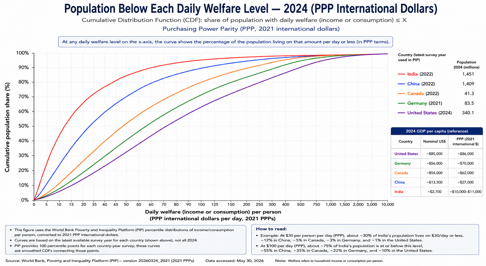
Figure 1. Population below each daily welfare level, PPP international dollars.
Note. This is a cumulative distribution function (CDF). The x-axis gives daily welfare—household income or consumption per person—expressed in PPP international dollars; the y-axis gives the cumulative percentage of the population at or below each level. The underlying World Bank Poverty and Inequality Platform (PIP) distributions are based on the latest available national survey observations rather than necessarily observed 2024 distributions for every country. PIP’s current release uses 2021 PPPs. The figure should therefore not be interpreted as a set of directly observed 2024 household-income distributions for all five economies (World Bank, 2026).
The figure provides a substantially different perspective from aggregate GDP.
At any point on the horizontal axis—for example, $10, $20, $50, or $100 per person per day—the corresponding point on each country’s curve indicates approximately what proportion of that population is at or below that daily welfare level.
India’s curve is concentrated strongly toward the lower end of the PPP income scale. China is substantially farther to the right, reflecting much higher welfare across a large share of its population. Germany, Canada, and the United States are farther to the right again.
This is the appropriate way to understand the apparent contradiction between a very large aggregate economy and comparatively low income per person. India can rank among the world’s largest economies in PPP terms while a large portion of its population remains at welfare levels that are low compared with advanced economies.
The same reasoning applies to China, although China’s distribution has shifted substantially upward over the past three decades.
The figure should not be confused with a Lorenz curve. It is a CDF of income or consumption, whereas a Lorenz curve shows the cumulative share of total income or consumption received by cumulative population and is used to visualize inequality and derive the Gini coefficient.
The latest nominal-dollar income distribution
The PPP figure should be read alongside the corresponding nominal-U.S.-dollar distribution, because the two measures answer different questions.
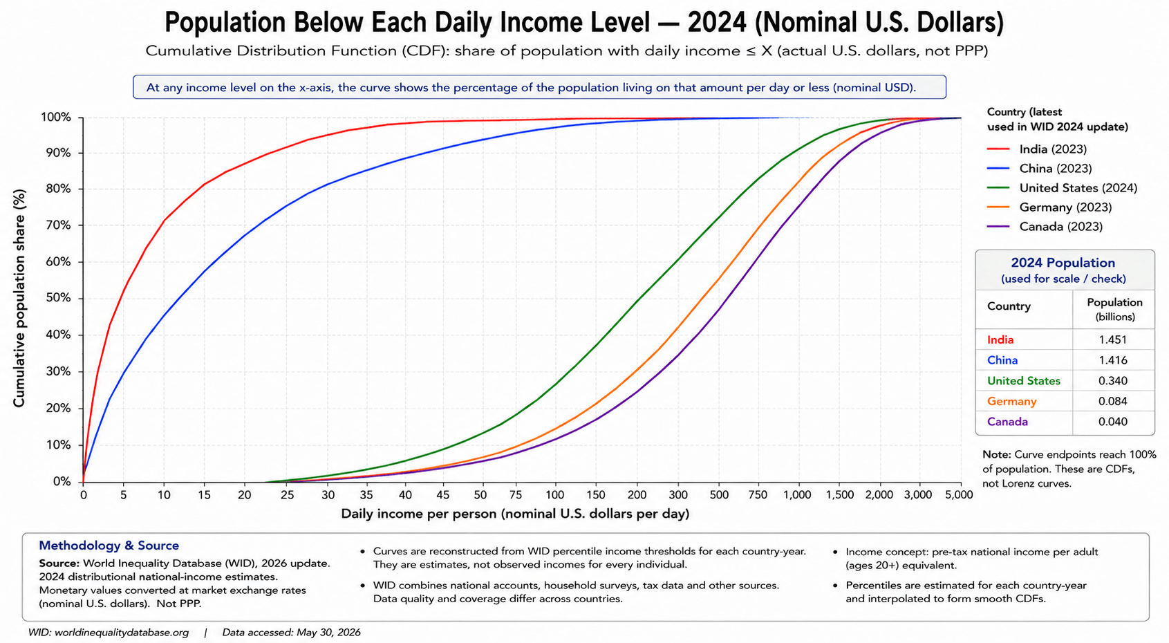
Figure 2. Population below each daily income level, nominal U.S. dollars.
Note. This cumulative distribution function uses estimated income distributions from the World Inequality Database (WID), expressed in nominal U.S. dollars using market exchange rates rather than PPP. WID’s distributional estimates are constructed from national accounts, surveys, fiscal data, and related sources and should be understood as estimates rather than observed income for every individual. The latest distribution year may differ from 2024 for some countries (World Inequality Database [WID], 2026).
The two figures should not produce the same curve because they measure the distribution in different units.
The PPP graph is more informative when asking what a given level of income can purchase within the country.
The nominal-dollar graph is more informative when asking how incomes compare after conversion at market exchange rates—for example, when thinking about internationally traded goods, international education, foreign investment, overseas consumption, imported products, or assets denominated in U.S. dollars.
The distinction is especially striking for India and China. Their distributions move substantially farther to the right after PPP adjustment because many domestic goods and services are cheaper than in the United States, Germany, or Canada.
That does not make a $10 PPP income equivalent to a $10 U.S.-dollar income. They represent different purchasing-power concepts.
What is a “good” or “bad” Gini?
The Gini coefficient is often presented as though it were a simple scorecard: low is good and high is bad. That is directionally useful but economically incomplete.
The World Bank defines the Gini index as a measure of how far the distribution of income—or, in some countries, consumption expenditure—departs from perfect equality. A Gini of 0 represents perfect equality, while 100 represents perfect inequality (World Bank, 2026).
A broad descriptive interpretation is:
| Gini | Broad reading | Interpretation |
|---|---|---|
| 0–30 | Relatively low inequality | Economic resources are comparatively evenly distributed |
| 30–40 | Moderate inequality | Significant differences exist across households |
| 40+ | High inequality | Large relative differences in income or consumption |
These bands are descriptive rather than universal thresholds. The World Bank uses a Gini above 0.4 as a broad threshold for high inequality in its monitoring framework, but the precise economic interpretation depends on national circumstances and the underlying data (World Bank, 2026).
A lower Gini is generally desirable when the objective is a more equal distribution of economic resources. Extreme inequality can restrict social mobility, create unequal access to education and opportunity, and produce large disparities in living standards.
But a Gini coefficient is not a measure of whether people are rich or poor.
Two countries can have the same Gini coefficient while having radically different income levels. A Gini of 30 in a low-income country does not mean citizens are economically better off than citizens of a high-income country with a Gini of 40.
Similarly, a country’s Gini can increase while poverty falls and living standards improve. The reason is that the Gini measures relative inequality, whereas poverty measures absolute welfare (World Bank, 2026).
Inequality across the five economies
The latest internationally comparable World Bank observations do not all correspond to 2024, so they should not be presented as a single-year 2024 ranking.
| Country | Latest World Bank Gini* | Approx. year | Broad position |
|---|---|---|---|
| India | 25.5 | 2022 | Lowest measured Gini |
| Canada | ~29.9 | 2022 | Relatively low |
| Germany | ~33.7 | 2021 | Moderate |
| China | ~36.0 | 2022 | Moderate-to-high |
| United States | 41.8 | 2024 | Highest among the five |
*The latest available observation is not the same calendar year for every country. Moreover, the underlying welfare concept differs: India’s figure is based on consumption data, whereas the measures for many advanced economies are income-based. The World Bank explicitly cautions that inequality data are not perfectly comparable across countries or years because household surveys differ in methodology (World Bank, 2026).
India’s current PIP profile reports a Gini of 25.51 for 2022, while China’s reports 36.02 for 2022. PIP reports 2024 populations of approximately 1.451 billion for India and 1.409 billion for China, meaning India had overtaken China in population by a substantial margin (World Bank, 2026).
India’s low Gini needs to be interpreted carefully
India’s latest World Bank Gini of approximately 25.5 is based on consumption expenditure, rather than the income-based approach predominantly used for the high-income economies. That distinction matters because consumption generally displays less inequality than income.
The World Bank’s recent analysis of India also identifies limitations in the underlying consumption data, particularly in capturing high-income households and their expenditures. Consequently, India’s latest consumption-based Gini should not be interpreted as proof that India has exceptionally equal income or wealth distribution (World Bank, 2026).
A more defensible statement is:
India has a relatively low measured consumption inequality according to the latest World Bank data, but that figure cannot be directly equated with an income or wealth inequality measure used for the United States, Germany, or Canada.
This distinction prevents a misleading conclusion that India is economically more egalitarian simply because its World Bank Gini is lower.
China’s inequality increased during its transformation
China’s experience is particularly instructive.
The World Bank series shows China’s Gini rising substantially during the country’s rapid industrialization and urbanization. Historical observations moved from the low-to-mid 30s during the 1990s toward above 40 during parts of the 2000s and early 2010s, before subsequently declining toward approximately 36 in 2022 (World Bank, 2026).
This does not mean China’s economic transformation was unsuccessful.
Quite the opposite: enormous numbers of people experienced substantial improvements in income, housing, infrastructure, and consumption while the distribution became more unequal for a period.
This is a classic example of why growth and equality must be measured separately.
An economy can generate enormous absolute gains while also producing a wider gap between groups.
The United States: richest per person, most unequal of the five
The United States presents the opposite combination.
Its nominal GDP per capita was approximately $85,000–$86,000 in 2024, vastly above India and China. Yet its World Bank Gini was approximately 41.8, above the latest observations for all four other countries (World Bank, 2026).
The U.S. therefore combines:
very high average output + high measured inequality.
This demonstrates why the Gini must never be interpreted as a proxy for national prosperity.
A society can be considerably more unequal while still having substantially higher average incomes and consumption possibilities.
The policy question is not simply whether inequality exists. It is whether inequality becomes sufficiently large to restrict opportunity, undermine social mobility, or prevent economic growth from translating into broadly shared improvements in living standards.
Canada and Germany occupy a middle position
Canada and Germany are instructive because both combine relatively high GDP per capita with lower measured inequality than the United States.
Germany’s latest World Bank Gini is around 33.7, while Canada’s is around 29.9, placing both substantially below the U.S. level (World Bank, 2026).
Canada therefore offers a combination of relatively high average income and comparatively low measured inequality.
Germany similarly combines high per-person output with moderate inequality, although its major economic problem has increasingly been weak growth rather than income distribution.
The comparison therefore produces five very different combinations:
United States: very high income + high inequality.
Germany: high income + moderate inequality + weak growth.
Canada: high income + relatively low inequality + weaker productivity growth.
China: rapidly rising income + moderate inequality + historically rising and subsequently declining inequality.
India: rapidly rising but still low income per person + low measured consumption inequality, with substantial measurement limitations.
Growth, inequality, and poverty are different questions
High economic growth does not automatically mean an economy has become more equal.
This is one of the most important lessons from the comparison.
China’s rapid industrialization raised national output and living standards enormously but was accompanied by increased inequality during important parts of the transformation. India has produced rapid economic growth while reporting comparatively low consumption inequality, although the measurement basis is different.
The United States has much higher average income but also substantially higher measured inequality.
The appropriate question is therefore not simply:
“Which country is more equal?”
It is:
“How much economic output does each person have, how widely are economic resources distributed, and how has that distribution changed as the economy has grown?”
Those are separate questions.
Inequality is not the same as poverty
This distinction deserves emphasis because it changes the interpretation of the entire thirty-year comparison.
Suppose average income increases from $10,000 to $20,000 while the Gini rises from 30 to 35. Inequality has increased, but average living standards may also have improved substantially.
Conversely, a country can have a low Gini while almost everyone remains poor.
Thus:
Gini = relative distribution.
GDP per capita = average economic output.
Poverty rate = proportion below a defined welfare threshold.
Median income = income of the person at the middle of the distribution.
These measures answer different questions.
The most meaningful assessment of economic progress therefore combines growth, per-person output, inequality, median income, and poverty rather than relying on any single indicator.
The long-term transformation in one table
Putting the major dimensions together produces a more complete picture:
| Country | 1995 economic position | 2024 economic position | Real-growth performance | 2024 nominal GDP/person | Latest Gini* |
|---|---|---|---|---|---|
| China | Much smaller, low-income economy | $18.7T nominal; largest by PPP | Very rapid | ~$13,300 | ~36.0 |
| India | Very small, low-income economy | $3.9T nominal; third-largest by PPP | Rapid | ~$2,700 | 25.5 |
| United States | Largest advanced economy | World’s largest nominal economy | Moderate/persistent | ~$85,000 | 41.8 |
| Germany | Large high-income economy | ~$4.7T nominal | Slow | ~$56,000 | ~33.7 |
| Canada | Smaller high-income economy | ~$2.2T nominal | Moderate but weakening | ~$54,000 | ~29.9 |
*Gini years differ by country and survey methodology.
This combined table reveals something that headline GDP rankings conceal.
China and India achieved the largest relative increases in economic size, but they remain much poorer per person than the advanced economies.
The United States remains dramatically richer per person but distributes that prosperity more unequally than the other four countries according to the latest World Bank Gini observations.
Germany has very high per-person output but weak economic growth.
Canada combines high per-person output and comparatively low measured inequality but has struggled to maintain strong productivity growth.
The importance of starting conditions
It is also misleading to interpret these growth rates without considering the countries’ starting points.
China and India began the period at dramatically lower income levels than the United States, Germany, and Canada. A large emerging economy can grow quickly through capital accumulation, urbanization, infrastructure development, industrialization, and movement of workers from low-productivity agriculture into higher-productivity sectors.
Germany, Canada, and the United States were already advanced economies in 1995. Their economies therefore faced diminishing returns to simply adding factories, workers, and infrastructure. Their challenge was to generate growth through productivity, innovation, human capital, and technological change.
This is why the difference between 6.3% and 2.5% should not be interpreted as meaning India is inherently more economically efficient than the United States. The countries have operated at different levels of development and under different demographic, institutional, and economic conditions.
The pandemic did not erase the underlying pattern
The 2020–2024 period could have dramatically altered the thirty-year rankings, but it did not.
India and China continued to expand more rapidly than the advanced economies after the pandemic. The United States demonstrated a strong recovery. Canada experienced weaker momentum, while Germany suffered prolonged stagnation (IMF, 2026; World Bank, 2025).
The pandemic therefore acted more as a stress test of existing economic structures than as a complete reset.
The IMF’s current assessment continues to show an uneven global outlook, with India projected well above China and the advanced economies, while Germany remains at the bottom of the five-country comparison (IMF, 2026).
The next thirty years
The next three decades may not reproduce the last.
China is already operating at a much slower growth rate than during its economic miracle. India must create enough productive employment and investment to sustain its expansion as its economy becomes larger. The United States must preserve its technological and productivity advantages while managing fiscal, demographic, and geopolitical pressures.
Canada must improve productivity so that population growth translates into stronger living standards rather than merely a larger aggregate economy.
Germany faces the most urgent need to rebuild its growth model around innovation, investment, energy security, industrial competitiveness, and productivity.
The IMF’s current forecasts nevertheless suggest that the broad ordering of growth may persist. India is projected to remain substantially faster-growing than China and the advanced economies, while Germany remains the weakest of the five in the near term (IMF, 2026).
These are forecasts rather than certainties. Wars, trade restrictions, technological change, commodity prices, demographic shifts, fiscal conditions, and monetary policy can substantially alter economic trajectories.
Conclusion
The past thirty years represent one of the most significant shifts in the global economic balance in modern history.
From approximately 1995 to 2024, China averaged about 8.4% real GDP growth annually and India approximately 6.3%, compared with roughly 2.5% for the United States, 2.4% for Canada, and 1.2% for Germany (IMF, 2026; World Bank, 2025).
The corresponding change in economic scale is even more striking. China’s nominal GDP rose from about $0.74 trillion to $18.74 trillion, while India’s increased from approximately $0.36 trillion to $3.91 trillion. At PPP, China’s 2024 economy reached approximately $38.19 trillion and India’s approximately $16.19 trillion, compared with roughly $29.18 trillion for the United States (World Bank, 2025).
But economic size tells only part of the story.
In nominal GDP per capita, the United States remains dramatically ahead, followed by Germany and Canada, while China has substantially surpassed India. PPP narrows these differences but does not eliminate them.
The distributional evidence adds another layer. The latest World Bank observations place the United States at approximately 41.8, China at 36.0, Germany at 33.7, Canada around 29.9, and India at 25.5 under its latest consumption-based observation. These figures are not all from 2024 and are not perfectly comparable because of differences in survey methodology and whether the underlying measure is income or consumption (World Bank, 2026).
The two income-distribution figures add another dimension. The PPP CDF shows where cumulative shares of each population are situated in terms of domestic purchasing power, while the nominal-dollar CDF shows how those same populations compare when income is converted using market exchange rates. Neither should be mistaken for GDP per capita or for a Lorenz curve; they illuminate different dimensions of economic life.
The combined picture is therefore more nuanced than the headline growth numbers.
China became enormously larger and substantially richer per person, but also more unequal than it was before its economic transformation.
India became dramatically larger and richer, although its average income remains far below that of the advanced economies. Its measured consumption inequality is relatively low, but methodological limitations make direct comparisons difficult.
The United States remains by far the richest of the five on a nominal per-person basis and the largest economy at market exchange rates, but it also has the highest measured inequality in this comparison.
Canada remains relatively affluent and relatively equal, but weaker productivity and per-capita growth are increasingly important concerns.
Germany remains wealthy and moderately equal but has experienced the weakest long-term growth and the most pronounced recent stagnation.
Ultimately, the economic transformation of the last thirty years cannot be understood through a single number.
Real GDP growth measures the speed of economic expansion. Nominal GDP measures market-value economic weight. PPP measures relative domestic purchasing power. GDP per capita measures average output relative to population. The Gini measures relative distribution. Poverty measures absolute deprivation. Income-distribution curves show how economic resources are distributed across the population.
Only by examining all of them together can the divergent economic experiences of India, China, Germany, Canada, and the United States be properly understood.
References
International Monetary Fund. (2026). World Economic Outlook database, April 2026. IMF Data.
https://data.imf.org/Datasets/WEO
International Monetary Fund. (2026). World Economic Outlook update, July 2026. International Monetary Fund.
https://www.imf.org/en/Publications/WEO/Issues/2026/07/08/world-economic-outlook-update-july-2026
World Bank. (2025). World Development Indicators. World Bank DataBank.
https://databank.worldbank.org/source/world-development-indicators
World Bank. (2025). GDP growth (annual %). World Development Indicators.
https://data.worldbank.org/indicator/NY.GDP.MKTP.KD.ZG
World Bank. (2025). GDP (current US$). World Development Indicators.
https://data.worldbank.org/indicator/NY.GDP.MKTP.CD
World Bank. (2025). GDP, PPP (current international $). World Development Indicators.
https://data.worldbank.org/indicator/NY.GDP.MKTP.PP.CD
World Bank. (2026). GDP per capita (current US$). World Development Indicators.
https://data.worldbank.org/indicator/NY.GDP.PCAP.CD
World Bank. (2026). GDP per capita, PPP (current international $). World Development Indicators.
https://data.worldbank.org/indicator/NY.GDP.PCAP.PP.CD
World Bank. (2026). Gini index. World Development Indicators.
https://data.worldbank.org/indicator/SI.POV.GINI
World Bank. (2026). Poverty and Inequality Platform.
https://pip.worldbank.org/
World Bank. (2026). India country profile. Poverty and Inequality Platform.
https://pip.worldbank.org/country-profiles/IND
World Bank. (2026). China country profile. Poverty and Inequality Platform.
https://pip.worldbank.org/country-profiles/CHN
World Inequality Database. (2026). World Inequality Database: Data and methodology.
https://wid.world/
World Inequality Database. (2026). World Inequality Report 2026.
https://wid.world/document/world-inequality-report-2026/